Deep Learning Explained: A Complete Practical Guide for Developers
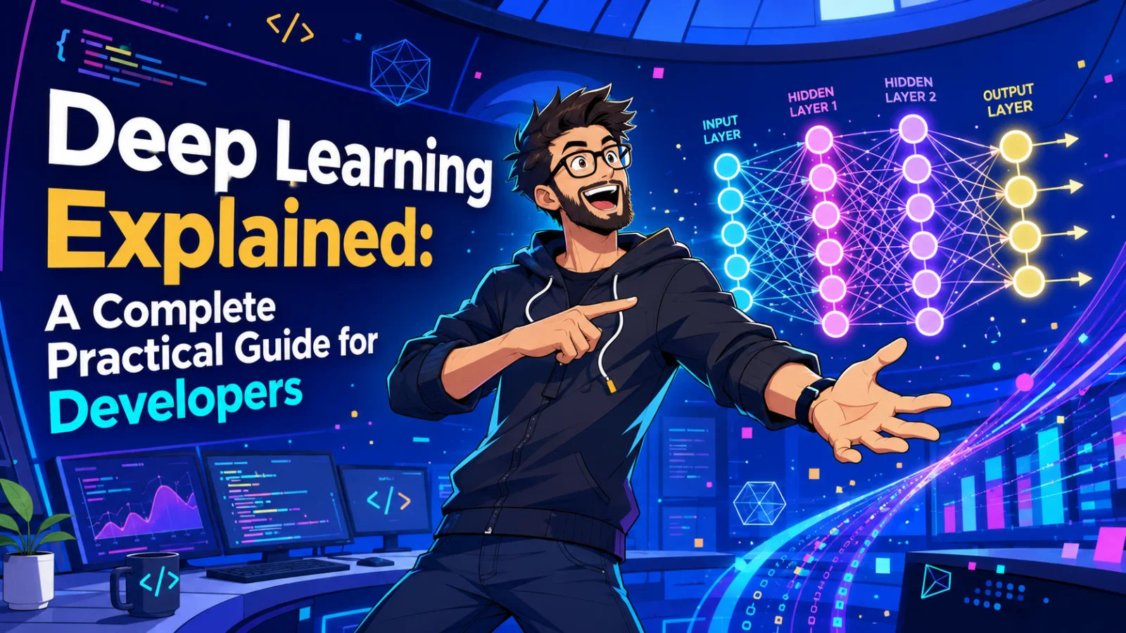
A developer-focused guide to how deep learning works—from neurons and gradient descent to CNNs, transformers, production deployment, and the questions engineers should be ready to answer.
Deep Learning Explained: A Complete Practical Guide for Developers
Deep learning is a branch of machine learning that uses neural networks with multiple layers to learn useful representations directly from data. Instead of asking an engineer to hand-design every feature, a deep model can discover increasingly abstract patterns: edges become shapes, shapes become objects, words become contextual meanings, and events become predictions.
This guide explains the ideas that matter in practice. It is designed for software developers who want a technically accurate mental model without beginning with advanced mathematics.
1. Artificial intelligence, machine learning, and deep learning
Artificial intelligence is the broad goal of building systems that perform tasks associated with human intelligence. Machine learning is a subset of AI in which systems learn patterns from examples. Deep learning is a subset of machine learning based mainly on multilayer neural networks.
Traditional machine-learning systems often depend on manually engineered features. A deep-learning system can learn many of those features automatically, but it usually needs more data, more computing power, and more careful monitoring.
2. The artificial neuron
A neuron receives input values, multiplies each one by a learned weight, adds a bias, and applies an activation function:
z = w1x1 + w2x2 + ... + wnxn + b
output = activation(z)
Weights determine the influence of each input. The bias shifts the decision boundary. The activation function introduces non-linearity; without it, stacking many layers would still behave like a single linear transformation.
Common activation functions include ReLU, which is fast and effective in hidden layers; sigmoid, often used for a binary probability; tanh, which produces values between -1 and 1; and softmax, which converts output scores into a multiclass probability distribution.
3. Layers and forward propagation
A feed-forward network normally contains an input layer, one or more hidden layers, and an output layer. During forward propagation, data moves from the input through every layer to produce a prediction.
Each hidden layer learns a representation useful to the next layer. Earlier layers tend to learn simple patterns, while deeper layers combine them into more complex concepts. “Deep” refers to this depth of learned transformations, not to consciousness or human-like understanding.
4. Loss functions: measuring error
Training needs a numerical objective. A loss function measures how different the prediction is from the correct target.
Mean squared error is common for regression. Binary cross-entropy is common for two-class classification. Categorical cross-entropy is common for multiclass classification. The correct loss must match both the task and the output layer. A model cannot improve reliably if its objective does not represent the real business goal.
5. Backpropagation and gradient descent
Backpropagation computes how much each parameter contributed to the error by applying the chain rule from the output layer back toward the input. It does not directly update the weights; it calculates gradients.
An optimizer then uses those gradients to update parameters:
new weight = old weight - learning rate × gradient
The learning rate is critical. If it is too large, training may oscillate or diverge. If it is too small, training can be unnecessarily slow or become stuck. Stochastic gradient descent is the classic optimizer. Adam adapts the learning rate for individual parameters and is a strong default, although SGD can generalize better in some workloads.
6. Epochs, batches, and the training loop
An epoch is one complete pass through the training set. A batch is the subset processed before one parameter update. The standard loop is: load a batch; run forward propagation; compute the loss; clear old gradients; run backpropagation; update the weights; repeat; then evaluate on validation data.
Small batches use less memory and introduce noisy gradients that can help generalization. Large batches improve hardware utilization but may require learning-rate changes.
7. Data preparation and splits
Model quality depends heavily on data quality. Remove corrupt examples, standardize labels, handle missing values, normalize numeric features, tokenize text correctly, and document every transformation.
Use separate training, validation, and test sets. The training set updates parameters. The validation set guides architecture and hyperparameter decisions. The test set is used only for the final unbiased estimate. Prevent data leakage: information from validation or test examples must never influence training features or preprocessing statistics.
For time-based problems, split chronologically. For grouped data, such as multiple records from one patient or customer, keep each group in only one split.
8. Overfitting and regularization
Overfitting occurs when a model memorizes training details but performs poorly on unseen data. Warning signs include falling training loss while validation loss rises.
Useful controls include more representative data, data augmentation, L1 or L2 weight penalties, dropout, early stopping, smaller models, and cross-validation. Batch normalization can stabilize optimization, while layer normalization is widely used in transformers. Regularization is not a substitute for fixing biased, duplicated, or leaked data.
9. Major deep-learning architectures
Fully connected networks are useful for fixed-size feature vectors and simple baselines.
Convolutional neural networks use learned filters and shared weights. They are efficient at detecting local spatial patterns and remain important for images, audio, and some time-series workloads.
Recurrent neural networks process sequences while carrying hidden state. LSTM and GRU units reduce the vanishing-gradient problem, though transformers have replaced recurrent models in many large-scale language tasks.
Transformers use self-attention to let each token weigh information from other tokens. They support parallel training and power modern language models, vision transformers, and multimodal systems. Attention is powerful but can be expensive because standard self-attention grows quadratically with sequence length.
Autoencoders learn to compress and reconstruct data. They are used for representation learning, denoising, and anomaly detection.
Generative adversarial networks train a generator against a discriminator. Diffusion models learn to reverse a noise process and are now widely used for high-quality image and media generation.
10. A minimal PyTorch example
A compact classifier with ten numeric inputs can be built with Linear(10, 64), ReLU, Dropout(0.2), Linear(64, 32), ReLU, and Linear(32, 2). During each training step, clear gradients, calculate logits, compute CrossEntropyLoss, call backward(), and let Adam update the parameters. CrossEntropyLoss expects raw logits, so do not apply softmax inside the model during training. PyTorch accumulates gradients by default, which is why they must be cleared before the next backward pass.
11. Evaluation beyond accuracy
Accuracy can be misleading when classes are imbalanced. For classification, inspect precision, recall, F1 score, confusion matrices, ROC-AUC, and PR-AUC. For regression, common metrics include MAE, RMSE, and R-squared.
Choose metrics based on the cost of mistakes. Fraud detection may prioritize recall while controlling false positives. Medical screening may treat missed positives as especially costly. Also evaluate calibration, subgroup performance, robustness, latency, memory usage, and cost per prediction.
12. Transfer learning and fine-tuning
Training from scratch is often unnecessary. A pretrained model has already learned reusable representations. Transfer learning replaces or adapts its final layers for a new task. Fine-tuning updates some or all pretrained parameters using a smaller task-specific dataset.
Start with a pretrained baseline, freeze most layers, train the new head, then gradually unfreeze layers if needed. Use a lower learning rate during fine-tuning to avoid destroying useful learned features.
13. From notebook to production
A production model is one component in a larger system. Version the dataset, code, configuration, weights, tokenizer, and evaluation results. Package preprocessing with inference so training and production transform data identically.
Expose the model through a synchronous API for interactive requests or a queue/batch pipeline for heavy workloads. Consider model size, CPU versus GPU cost, batching, caching, quantization, and autoscaling.
Monitor input drift, prediction drift, latency, error rates, resource use, and real-world outcome metrics. Keep rollback capability. Retraining should be a controlled pipeline with validation gates, not an automatic reaction to every change.
14. Security, privacy, and responsible use
Training data can contain personal, licensed, biased, or malicious content. Apply data minimization, access control, encryption, retention policies, and provenance tracking. Test for bias across relevant groups. Protect inference endpoints against abuse, oversized requests, model extraction, and adversarial inputs.
Deep models produce statistical predictions, not guaranteed truth. High-impact decisions need human oversight, transparent limitations, audit logs, and a safe appeal process.
15. Common mistakes developers make
Starting with a huge model before building a simple baseline; optimizing accuracy while ignoring the real cost of errors; evaluating repeatedly on the test set; allowing duplicate or future data to leak across splits; applying different preprocessing in training and production; assuming lower training loss always means a better product; ignoring latency and cloud cost until launch; deploying without drift monitoring, rollback, or versioning; and treating generated output as factual without verification.
16. A practical project plan
For an image classifier, begin with a clear label policy and a small audited dataset. Build a simple pretrained baseline. Create train, validation, and test splits before experimentation. Add augmentation only to training data. Track every experiment and compare it against the same metrics.
After choosing a model, export it, write an inference service, add input validation, and load-test the endpoint. Deploy to a small percentage of traffic. Monitor quality and operational metrics, then expand gradually. This staged approach reduces both technical and product risk.
17. Deep-learning interview questions
What is the difference between a parameter and a hyperparameter? Parameters, such as weights and biases, are learned during training. Hyperparameters, such as learning rate, batch size, and layer count, are selected by engineers or tuning systems.
Why are activation functions needed? They introduce non-linearity, allowing a network to learn complex relationships.
What is the vanishing-gradient problem? Gradients can become extremely small as they move backward through many layers, slowing or preventing learning in early layers.
Why separate validation and test data? Validation guides choices; the untouched test set estimates final generalization.
What does dropout do? During training it randomly disables some activations, discouraging fragile co-adaptation.
What is data leakage? It is the accidental use of information during training that would not be available at prediction time.
When would you use transfer learning? When a suitable pretrained model exists and the task-specific dataset or compute budget is limited.
Why can accuracy be a bad metric? A model can achieve high accuracy by predicting the majority class while failing on important minority cases.
What is the difference between inference and training? Training adjusts parameters using gradients. Inference uses fixed parameters to generate predictions.
How do you know a model is production-ready? It must meet quality, fairness, robustness, latency, reliability, cost, security, observability, and rollback requirements—not only an offline score.
Conclusion
Deep learning is not magic. It is an engineering discipline built on data, differentiable models, optimization, disciplined evaluation, and reliable production systems. Learn the forward pass, loss, backpropagation, and data-splitting fundamentals first. Then explore specialized architectures. The best deep-learning solution is not the largest model; it is the simplest system that delivers measurable value safely and reliably.
Featured Articles

8 Claude Code Plugins That Make Everyday Development Easier in 2026
A practical shortlist of Claude Code plugins, with real use cases and a sensible way to start.

Laravel 13 AI SDK: Build a Useful First Agent Without Losing Control
A practical introduction to Laravel’s first-party AI SDK, using support-ticket triage to show where an agent helps and where application code stays in charge.

YOLO Object Detection: A Complete Practical Guide for Developers
A developer-focused, end-to-end guide to YOLO object detection covering core concepts, datasets, training, evaluation, real-time inference, deployment, optimization, production risks, and interviews.
Comments
0 commentsNo approved comments are visible yet. New community replies may wait for moderation.